type
status
date
slug
summary
tags
category
icon
password
Background
The mechanics of our ear convert sound into vibrations of the basilar membrane. The way this works:


This means that our ear automatically performs approximately a Fourier Transformation on the incoming sound, separating the high frequency compents from the low frequency components. This feature is used in the extremely successful design of cochlea implants (CIs): There sound is separated into approximately 20 frequency bins, and 20 electrodes stimulate the corresponding auditory nerve cells:

Limitation of CI-Electrodes

Possible Solutions: Time Domain or Frequency Domain

(a) Time Domain: Linear Filters - Gamma Tones
In fact, the basilar membrane does not behave like a Fourier Transform. To a first approximation, Gamma tones describe the frequency response of the basilar membrane quite well. They can be well -- and very efficiently -- be approximated by IIR-Filters. Note the "Multi-resolution behavior" of the gamma tones: high frequencies decay at a much faster (time)scale than the lower frequencies:

(b) Frequency Domain: Powerspectrum
One way to characterize the frequency dependence of a signal is to use a Fourier Transformation (FFT).
- The equation for the frequency components of an FFT is , where "N" is the number of data-points, "Ts" the sampling-interval, and "n" the running index (1:N)
- Frequencies on the basilar membrane are arranged approximately logarithmically. Take this fact into consideration.
Exercise Description: Simulation of Cochlea-Implants
Write a function that simulates cochlea implants:
- Your function should allow the user to interactively (=graphically) select an audio-file.
- Your function should produce as output a WAV-file, containing the CI-simulation corresponding to the selected audio-file.
- The simulated CI should have approximately the following specifications:
- = 200 Hz
- = 500 - 5000 Hz
- numElectrodes = 20
- StepSize = 5 - 20 ms
- Provide your program with an option to try out the n-out-of-m strategy used in real cochlear implants: at any given time, only those n (typically 6) of all m available (typically around 20) electrodes are activated, which have the largest stimulation.
Possible Program Structure:
- Select file
- Read data (mp3, wav)
- Set parametersnumber of electrodesfrequency rangeWindow size (sec)[Window type][sample rate]
- [CalculateWindow size (points)Electrode locations]
- Allocate memory
- For [all data]Get dataCalculate stimulation strengthSet/write output values
- Play result

Implementation
In the implementation, we strictly follow the principles which have been mentioned before.
Read in the data
First, we need to read in the original sound. In order to process the data more easily, we take the average of multiple channels.
# Read data.
sound = sounds.Sound()
if len(sound.data.shape) > 1:
    # Average on multiple channels.
    sound.data = np.mean(sound.data, axis=1)
Parameter settings
We set the parameters according to the suggestions in the document of requirements. To make the parameter setting more modularized, we set the parameters in a YAML file and create a class to structurally contain the parameters. The parameter settings are:
ex1:
  m_electrodes: 22  # Total number of electrodes
  n_channels: 9  # Number of activated channels
  lo_freq: 200  # Hz
  hi_freq: 5000  # Hz
  period_window: 6.0e-3  # sec
  step_window: 5.0e-4  # sec
  type_window: 'moore'  # Filter window type
What’s more, we also create a graphical interface to allow the users change the parameters interactively.
# Set parameters. Load the parameters from a YAML script.
path_crt = os.getcwd()
Params = Params_audio(path_options=os.path.join(path_crt, 'options.yaml'))

# Create a graphical interface to visualize and change the parameter settings.
Params = gui_params(Params=Params)

# Calculate other parameters.
size_window = round((Params.period_window/sound.duration)*sound.totalSamples)  # window size (points)
size_step = round((Params.step_window/sound.duration)*sound.totalSamples)  # step size (points)
Apply filters to the original audio
In this process, we set up a series of IIR filter banks and then apply them to the original audio. Next, we simulate the n-out-of-m strategy. The principle is, during the proccessing time, only n (which have the strongest stimulations) out of m electrodes (all available electrodes) will be activated. In this way, we need to calculate the signal intensities of each electrode and only select a part of them to activate. Then, we need to calculate the corresponding amplitudes for the subsequent signal reconstruction process.
# Set up IIR filter banks.
(forward, feedback, fcs, ERB, B) = GTS.GT_coefficients(
    fs=sound.rate, n_channels=Params.m_electrodes,
    lo_freq=Params.lo_freq, hi_freq=Params.hi_freq, method=Params.type_window
    )

# Apply filter banks on the whole audio.
data_filtered = GTS.GT_apply(sound.data, forward, feedback)

# Simulate the n_out_of_m process.
amp_n_out_m = n_out_m(
    data_audio=data_filtered, size_window=size_window,
    size_step=size_step, Params=Params
    )
Audio reconstruction
After the process of n-out-of-m strategy, we get the amplitudes of each frequency band during a time period. In order to reconstruct the output audio, we can make use of sine/cosine functions with these specific amplitudes. After generating sine/cosine functions, add them linearly to get final result.
# Audio reconstruction.
y_output = reconstruction(
    amps=amp_n_out_m, size_step=size_step, totalSamples=sound.totalSamples,
    duration=sound.duration, fcs=fcs
    )
# Write to output file
sound_output = sounds.Sound(inData=y_output, inRate=sound.rate)
sound_output.write_wav(full_out_file=os.path.join(path_crt, 'output.wav'))
Demo
Here we present several examples of the simulation results. We use two original sounds provided by the requirement document and compare them with the reconstruction outputs. The parameter settings are the same with as before.
tiger.wav
- Original:
- Simulation:
scales.wav
- Original:
- Simulation:
harmony.wav
- Original:
- Simulation:
According to the results of comparison, we can conclude that our simulation results can reconstruct the original sounds with a relatively low quality. One of the reasons is that we apply the n-out-of-m stategy during the simulation process. So only several frequency bands are activated.
In the interest of brevity, we only present the main structure of the simulation process. The source code can be found in my GitHub.
- 作者:Shuo Li
- 链接:https://shuoli199909.com/article/eth-cs-ex1
- 声明:本文采用 CC BY-NC-SA 4.0 许可协议,转载请注明出处。